Tutorial for DCGAN with Chainer
DCGAN: Generate the images with Deep Convolutional GAN
0. Introduction
In this tutorial, we generate images with generative adversarial network (GAN). It is a kind of generative model with deep neural network, and often applied to the image generation. The GAN technique is also applied to PaintsChainer a famous automatic coloring service.
In the tutorial, you will learn the following things:
- The basic idea of generative model
- The difference among GAN and other generative models
- Generative Adversarial Networks (GAN)
- Implementation of DCGAN in Chainer
1. The basic idea of generative model
1.1 What is the Model?
In the field of science and engineering, we describe a system using mathematical
concepts and language. The description is called as a mathematical model,
and the process of developing a mathematical model is mathematical modeling.
Especially, in the context of machine learning, we explain a target model by a
map from an input
to an output
\begin{align*} f: x \mapsto y \end{align*}
Therefore, the purpose of model training is obtaining the map from training data.
In the case of unsupervised learning, we use the dataset of inputs
as the training data,
and create the model
.
In supervised learning, we use the dataset of inputs and their outputs
. As a simple example,
let's consider a supervised learning problem such as classifying images into
dogs or cats. Then, the training dataset consist of input images
and their labels
.
1.2 What is the Generative Model?
When we think about the generative model, it models the probability distribution
which generates the training data
. The one of
most simple ideas is that the generative model models the probability distribution
with the map
. We assign each
and
of
as follows.
: the training data
: the likelihood of generating the training data
In the case, because we model the probability distribution explicitly,
we can calculate the likelihood
. In this situation, we can often optimize
the parameters of
to maximize the likelihood, and train the model with
maximum likelihood estimation.
So, there is an advantage that the training process is simple because you can just
maximize the likelihood by optimizing the parameters. However, there is a
disadvantage that we have to make a mechanism for sampling because we have only
the way of calculating the likelihood.
In the first place, we often just want to sample
according to the distribution in practice. The likelihood
is used
only for model training. In the case, we sometimes do not model the probability distribution
directly, but other targets to facilitate sampling.
There are two approaches to model the probability distribution .
The first case is to model the probability distributions
and
by introducing the latent variable
. The VAE, which is described later,
belongs to this category.
Second, we introduce the latent variable
and model the sample generator
]s = G(z)] which fits the distribution
. The GAN belongs to this category.
These models can generate the training data
by generating
the latent variable
based on random numbers.
These generative models can be used for the following purposes:
- Assistance for creative activities (e.g. coloring of line drawings)
- Providing interfaces to people (e.g. generating natural sentences)
- Reduction of data creation cost (e.g. use as a simulator)
Note
When we talk about generative model, we sometimes explain it against discrimination
model in classification problem [1]. However, when we talk about generative
model in GAN, it is natural to define it as a model of probability distribution
that generates training data.
2. The difference among GAN and other generative models
As explained in the GAN tutorial in NIPS 2016 [2], the generative models can be classified into the categories as shown in the following figure:
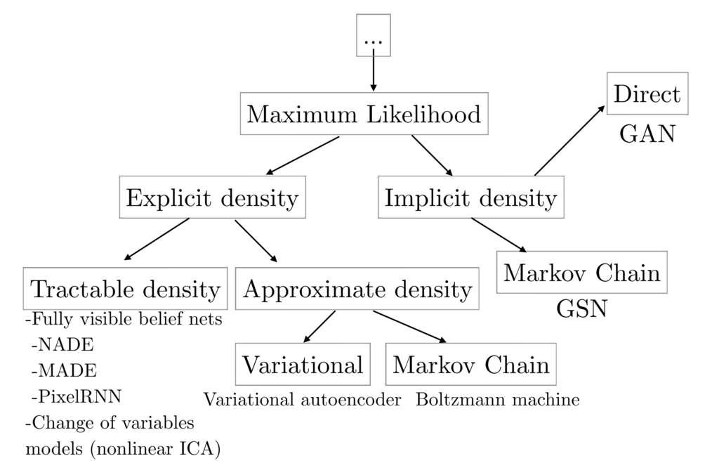
cited from [1]
Besides GAN, other famous generative models are Fully visible belief networks (FVBNs) and Variational autoencoder (VAE).
2.1 Fully Visible Belief Networks (FVBNs)
FVBNs decomposes the probability distribution into one-dimensional probability distributions
using the Bayes' theorem as shown in the following equation:
\begin{align*} p_{\mathrm{model}}({\bf s}) = \prod^{n}_{i=1}p_{\mathrm{model}} (s_i | s_1, \cdots, s_{i-1}) \end{align*}
Since the dimensions from , excluding the first dimension
, are
generated based on the dimensions previously generated, FVBNs can be said to be an autoregressive model.
PixcelRNN and PixcelCNN, which are categorized as FVBNs, model one-dimensional distribution functions
with Recurrent Neural Networks(RNN) and Convolutional Neural Networks(CNN), respectively.
The advantage of FVBNs is that the model can learn with explicitly computable likelihood.
The disadvantage is that the sampling cost can be expensive because each dimension can only be generated sequentially.
2.2 Variational Auto-Encoder (VAE)
The VAE models the probability distribution that generates the training data as follows:
\begin{align*} p_{\mathrm {model}}({\bf s}) = \int p_{\mathrm {model}}({\bf s}|{\bf z}) p_{\mathrm {model}}({\bf z}) d{\bf z} \end{align*}
is modeled by the two probability distributions
and
using the latent variable
.
When training a model using the maximum likelihood estimation on ,
we should calculate
or
explicitly. However, because
includes integral operator as
shown in above equation, it is difficult to calculate
and
.
So, VAE approximates with
.
As a result, we can calculate the lower bound of the likelihood,
and train the model by maximizing the lower bound of the likelihood. The advantage of VAE is
that sampling is low cost, and you can estimate latent variables by
.
The disadvantage is that calculation of the probability distribution
is difficult, and approximate values are used for training model.
3. Generarive Adversarial Networks (GAN)
3.1 What is the GAN?
Unlike FVBNs and VAE, GAN does not explicitly models the probability distribution
that generates the training data. Instead, we model a generator
.
The generator
samples
from the latent variable
.
Apart from the generator
, we create a discriminator
which identified the samples from the generator
and the true samples from training data.
While training the discriminator
, the generator
is also trained so that
th generated samples cannot be identified by the discriminator.
The advantages of GAN are low sampling cost and state-of-the-art in image generation.
The disadvantage is that we cannot calculate the probability distribution
because we do not model any probability distribution,
and we cannot infer the latent variable
from a sample.
3.2 How the GAN works?
As explained above, GAN uses the two models, the generator and the discriminator. In other words, we set up two neural networks for GAN.
When training the networks, we should match the distribution of the samples
generated from the true distribution with the distribution of the samples
generated from the generator.
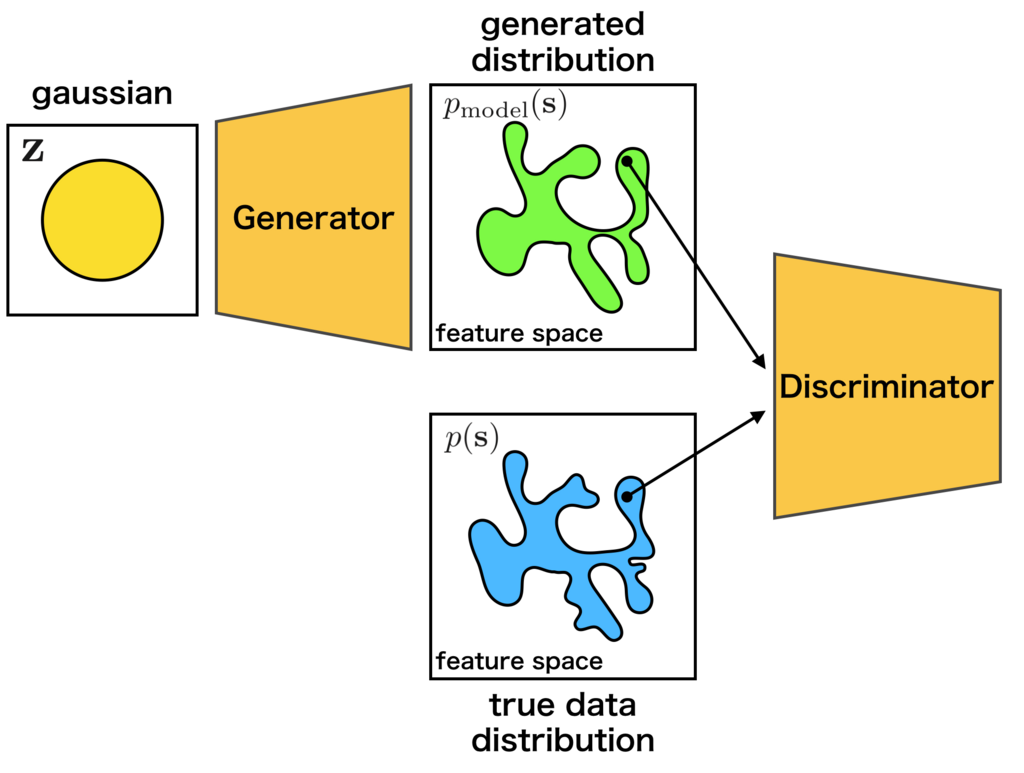
The generator learns the target distribution on the idea of
Nash equilibrium [3] of game theory.
In detail, while training the discriminator
,
the generator
is also trained so that the discriminator
cannot identify the generated samples.
As an intuitive example, the relationship between counterfeiters of banknotes and police is frequently used. The counterfeiters try to make counterfeit notes that are similar to real banknotes. The police try to distinguish real bank notes from counterfeit notes. It is supposed that the ability of the police gradually rises, so that real banknotes and counterfeit notes can be recognized well. Then, the counterfeiters will not be able to use counterfeit banknotes, so they will build more similar counterfeit banknotes to real. As the police improve the skill further, so that they can distinguish real and counterfeit notes... Eventually, the counterfeiter will be able to produce as similar banknote as genuine.
The training process is explained by mathematical expressions as follows.
First, since the discriminator is a probability
that the sample
is generated from the true distribution,
it can be expressed as follows:
\begin{align*} D({\bf s}) = \frac{p({\bf s})}{p({\bf s}) + p_{\mathrm{model}}({\bf s})} \end{align*}
Then, when we match the distributions of
the samples generated from true distribution
and the samples
generated from the generator
,
it means that we should minimize the dissimilarity between
the two distributions.
It is common to use Jensen-Shannon Divergence
to measure the dissimilarity between the distributions[4].
The of
and
can be written as follows by using
:
\begin{align*} 2 D_{\mathrm{JS}} &=& D_{\mathrm{KL}}(p(x)||\bar{p}(x)) + D_{\mathrm{KL}}(p_{\mathrm{model}}(x)||\bar{p}(x)) \\ &=& \mathbb{E}_{p(x)} \log \frac{2p(x)}{p(x) + p_{\mathrm{model}}(x)} + \mathbb{E}_{p_{\mathrm{model}}} \log \frac{2p_{\mathrm{model}}(x)}{p(x) + p_{\mathrm{model}}(x)} \\ &=& \mathbb{E}_{p(x)} \log D(x) + \mathbb{E}_{p_{\mathrm{model}}} \log (1-D(x)) + \log 4 \end{align*}
The will be maximized by the discriminator
and minimized by
the generator
, or
.
And the distribution
generated by
can match the true distribution
.
\begin{align*} \min_{G} \max_{D} \mathbb{E}_{p(x)} \log D(x) + \mathbb{E}_{p_{\mathrm{model}}} \log (1-D(x)) \end{align*}
When training actually, the above min-max problem is solved by alternately updating the
discriminator and the generator
[5].

cited from [5]
3.3 What is DCGAN?
In this section, we will introduce the model called DCGAN(Deep Convolutional GAN) proposed by Radford et al.[6]. As shown below, it is a model using CNN(Convolutional Neural Network) as its name suggests.
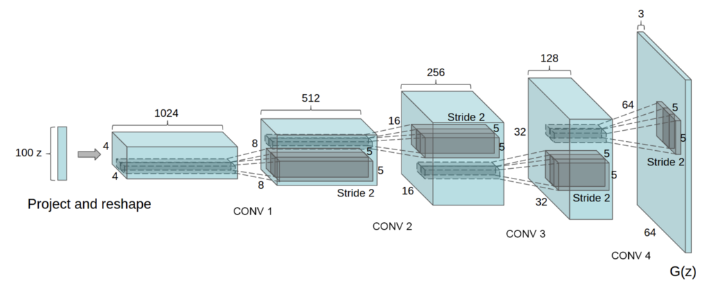
cited from [6]
In addition, although GAN is known for its difficulty in learning, this paper introduces various techniques for successful learning:
- Convert max-pooling layers to convolution layers
- Convert fully connected layers to global average pooling layers in the discriminator
- Use batch normalization layers in the generator and the discriminator
- Use leaky ReLU activation functions in the discriminator
4. Implementation of DCGAN in Chainer
There is an example of DCGAN in the official repository of Chainer, so we will explain how to implement DCGAN based on this: chainer/examples/dcgan
4.1 Define the generator model
First, let's define a network for the generator.
When we make a network in Chainer, we should follow some rules:
- Define a network class which inherits
chainer.Chain. - Make
chainer.links's instances in theinit_scope():of constructor__init__. - Concatenate
chainer.links's instances withchainer.functionsto make whole network.
If you are not familiar with constructing a new network, you can read this tutorial.
As we can see from the constructor __init__, the Generator
uses the deconvolution layer chainer.links.Deconvolution2D
and the batch normalization chainer.links.BatchNormalization.
In _call__, each layer is concatenated by chainer.functions.relu
except the last layer.
Because the first argument of L.Deconvolution is the channel size of input and
the second is the channel size of output, we can find that each layer halve the
channel size. When we construct Generator with ch=1024, the network
is same with the image above.
Note
Be careful when you concatenate a fully connected layer's output and
a convolutional layer's input. As we can see the 1st line of  ``__call__ ``,
the output and input have to be concatenated with reshaping by
``chainer.functions.reshape``.
4.2 Define the discriminator model
In addtion, let's define a network for the discriminator.
The Discriminator network is almost same with the transposed network
of the Generator. However, there are minor different points:
- Use
chainer.functions.leaky_reluas activation functions - Deeper than
Generator - Add some noise when concatenating layers
4.3 Prepare dataset and iterator
Let's retrieve the CIFAR-10 dataset by using Chainer's dataset utility function
chainer.datasets.get_cifar10. CIFAR-10 is a set of small natural images.
Each example is an RGB color image of size 32x32. In the original images,
each component of pixels is represented by one-byte unsigned integer.
This function scales the components to floating point values in
the interval [0, scale].
4.4 Prepare model and optimizer
4.5 Prepare updater
4.6 Prepare trainer and run
4.7 Start training
We can run the exemple as follows.
$ pwd
/root2chainer/chainer/examples/dcgan
$ python train_dcgan.py --gpu 0
GPU: 0
# Minibatch-size: 50
# n_hidden: 100
# epoch: 1000

epoch       iteration   gen/loss    dis/loss  ................]  0.01%
0           100         1.2292      1.76914
     total [..................................................]  0.02%
this epoch [#########.........................................] 19.00%
       190 iter, 0 epoch / 1000 epochs
    10.121 iters/sec. Estimated time to finish: 1 day, 3:26:26.372445.
The results will be saved in the director /root2chainer/chainer/examples/dcgan/result/.
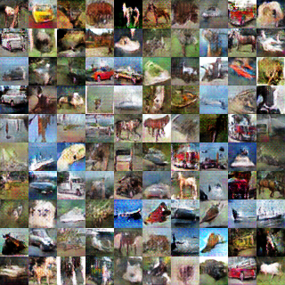
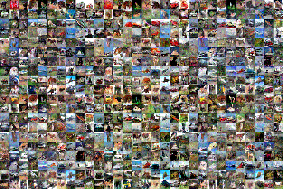
The image is generated by the generator trained with 1000 epochs, and the GIF image
on the top of this page shows generated images at the each 10 epoch.
